Learning SAS With Baseball Data, Where Process > Results

Last Monday marked the beginning of the “bootcamp” portion of the MSA program. Aside from two communications classes and preparing for a group presentation, the first week of bootcamp mainly consisted of learning and applying statistical concepts and the SAS programming language.
As a member of the orange summer cohort, I’ve spent my mornings attending lectures on SAS syntax and following a self-paced e-learning module. My afternoons consist of attending lectures on fundamental statistical concepts and how to apply them within SAS. A lab assignment accompanies each lecture and is meant to assess our understanding of the material covered in class. The lab assignments are relatively straightforward – we’re given a very specific set questions related to a certain set of data.
While I’ve found the lab assignments to be useful in reinforcing my understanding of the core programming and statistical concepts, I know that the upcoming practicum project (and most real-world analytics problems) will be much more open-ended. In order to prepare for those types of assignments, I spent some time after class exploring a few of the basic datasets included within the SAS software suite, without any agenda or predetermined set of questions.
As a lifelong baseball fan, the dataset that immediately caught my eye was simply titled “baseball.” I started my self-assigned project the same way I had started all the lab assignments – exploring the structure and contents of the data with the contents and print procedures.
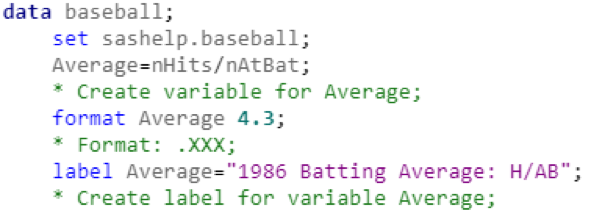
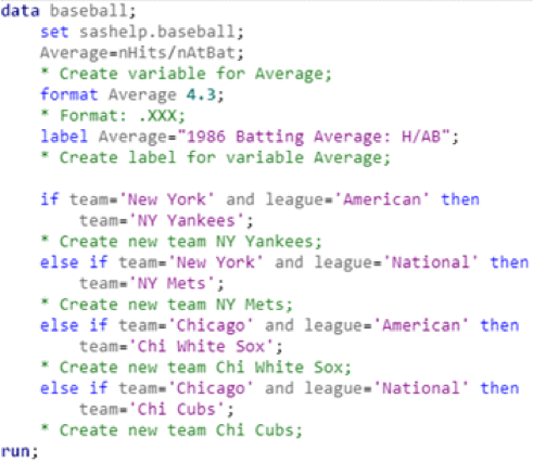
From the variable labels in the output, I determined that the data covered position player statistics from the 1986 MLB season (in hindsight, a particularly difficult season for me as a Red Sox fan, even though I was born in 1993). The data table includes 322 rows representing individual players, and 24 variables representing statistics for each player. The very first thing I noticed about the variables was that they did not include the most ubiquitous baseball statistic: batting average. Creating a new variable for batting average was fairly simple:

After sorting the data by “Average” in descending order, we can see the MLB leaderboard for batting average in 1986:

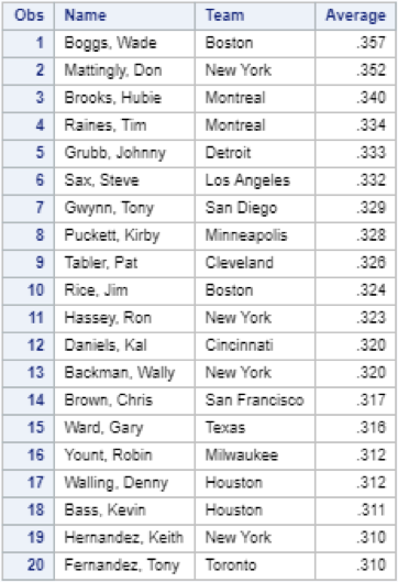
I’ll take this opportunity to point out that there are two Red Sox players (and members of the Hall of Fame) in the top ten. Now that I had calculated and sorted the batting averages for each player, the next logical step was to calculate batting average for each team. It was at this point that I really began to test the limits of my SAS knowledge. My initial thought was to use the means procedure, with the Team variable as the classifier:


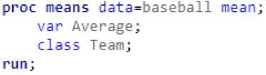
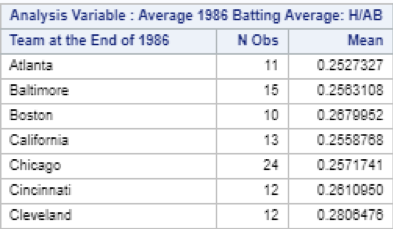
I realized that these results were inaccurate after thinking about the math for a few seconds. SAS was taking a simple average of several averages, but I was really trying to calculate a weighted average. If one player had 6 hits in 10 at-bats (.600 average) and another player had 6 hits in 20 at-bats (.300 average), they would be have a combined 12 hits in 30 at bats (.400 average). But using the code snipped above, SAS would simply calculate the average of .600 and .300 and return a batting average of .450. I spent quite a bit of time looking through SAS syntax documentation and online forums to find a solution for my weighted average problem. Eventually, I found a (somewhat indirect) way to achieve my intended result:

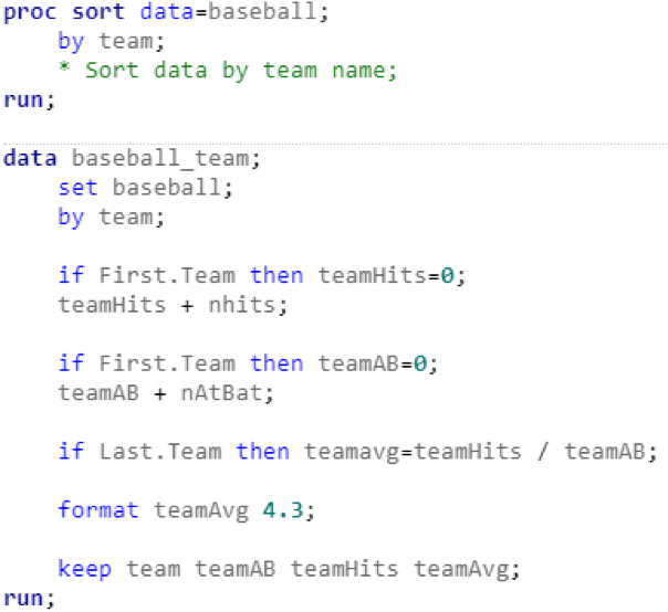
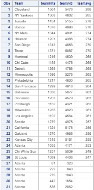
The sort procedure sorts the original table alphabetically by team name. The data step creates a new table, “baseball.team,” with three new variables: “teamAB,” “teamHits,” and “teamAvg.” Every time SAS encounters a new team, the variables “teamAB” and “teamHits” are reset to 0. Then, teamAB and teamHits increase by the amount of at-bats and hits for each player on that team. Once SAS reaches the last player on a given team, the total team average is calculated. I’ll admit that I was pretty excited to see the results:


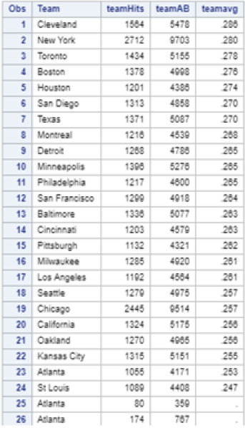
And I was immediately disappointed, as there were two glaring issues with my fancy new table.  First, based on my understanding of modern Major League Baseball, there should have been 30 unique teams, not 24. I looked up the official stats for the 1986 season and discovered there were actually only 26 teams in 1986. It didn’t take long to identify the problem. The “Team” variable includes only each team’s home city, but New York and Chicago each had two teams. It seems I rushed through the data exploration step at the beginning of my project and overlooked this issue. Luckily, there was an easy fix:

With the first issue solved, I turned my attention to the second issue. Although there were only 26 unique teams, my baseball.team data table still had 322 observations. After the 26 teams were displayed, there were 296 rows of empty data sorted alphabetically by team:

Again, I found a simple solution after a few minutes of deliberation:


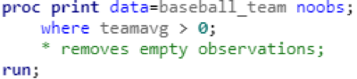
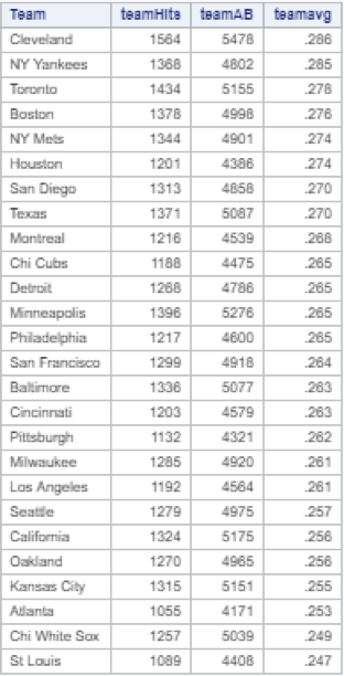
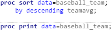
And there you have it. After much trial and error, I had achieved my desired result: a simple ranking of each team in order of descending batting average. Now of course this result is not particularly useful to anyone – the information above is readily available online. And the data above is not representative of actual team performance in 1986, for two reasons. First, since my original data table only included statistics for 322 players, my table does not reflect the full team batting averages for the 1986 season. Additionally, each player’s team is listed as the team that they ended the 1986 season with, so if a player changed teams during the season their statistics would all be attributed to their final team, and not necessarily the team that they played for at the time.
However, the process was immensely entertaining and valuable to me from an educational perspective. I got to practice several of the SAS statements I had learned in class up to that point, and even learned a few new ones along the way. I also learned some valuable lessons about carefully examining data before beginning to manipulate it. I talked through the issues I encountered with several fellow students, as well as a professor who provided much more elegant solutions than the ones I had come up with on my own.
I really enjoyed the process of working through the problems that I encountered while exploring this dataset, and I can’t wait to apply the lessons I learned in R, Python, and SQL when we start using them this fall.
Columnist: Kevin McDowell